


The short version. Robotics simulation tests a robot's behaviour in software, using models of the robot, its sensors and its environment instead of physical hardware. It is cheaper, faster and safer than testing on real robots, but behaviour that works in simulation still has to be proven on hardware. Simulating a robotic arm takes a simulator such as Gazebo, ROS 2 to connect the components, a planner such as MoveIt 2, and controllers from ros2_control.
A robotics project usually moves through four stages: define the task, develop and test the behaviour in simulation, transfer it to real hardware, then deploy and maintain it in operation. Simulation comes early, often before the hardware has been chosen, because it is the cheapest way to find out what works.
This article covers the first two stages. The task is a simple demonstration: pick and place with two robotic arms across two moving conveyor belts. We build up to it in steps, starting with one arm that places an object in a box. The transfer to real hardware is outside the scope of this article.
Why do we simulate robots?
Experimenting with robots comes with several challenges:
- Robots are expensive. Working with robots requires costly hardware, props and sensors. They also take up a lot of space: a land robot requires test tracks, a drone a large outdoor flying facility.
- Robots are slow. Reaching the desired behaviour takes thousands of trials, stress tests under extreme conditions, and repeated runs to ensure consistency and reliability. Every aspect needs to be tested independently, which requires full control over the environment and several tests under varying conditions. Every run takes minutes or hours; even the easiest problems would take months of attempts.
- Robots are dangerous. If not controlled properly, they risk damaging property or themselves, or causing harm to people.
All these issues can be avoided (or greatly reduced) with simulation.
Modern simulation frameworks model the physics of the real world, the hardware and its operating conditions, inside a self-contained environment. The main running cost is compute. Before committing to hardware, digital versions of various models can be tested and compared.
Simulations can run in parallel and faster than real time, compressing months of attempts into a couple of days. Every aspect of the environment can be controlled: variables can be isolated from each other, and extreme conditions and corner cases are easy to replicate. All of this comes with no risk of harm or damage.
The gap
However, behaviour that works in simulation doesn't automatically work on a real robot.
The physics engine, the environment, the sensors and the hardware are all imperfect approximations of reality. Simulation time is discrete, and can't capture the real timing of events. This gap between simulation and reality is why setups that pass thousands of simulated experiments can still fail the first time they run on real hardware.
Simulation narrows down what needs to be proven in the real world, but it doesn't remove the need to prove it.
The first step: pick and place with one arm
What does it take to simulate a robotic arm that picks up an object and puts it in a box? We start with this simple scenario:
- A UR3e robotic arm with 6 joints
- A Robotiq 2F-85 gripper
- A pill-shaped object
- A rectangular box
We run it on ROS 2 Jazzy, Gazebo Harmonic, MoveIt 2 and ros2_control, each explained below.
The control loop
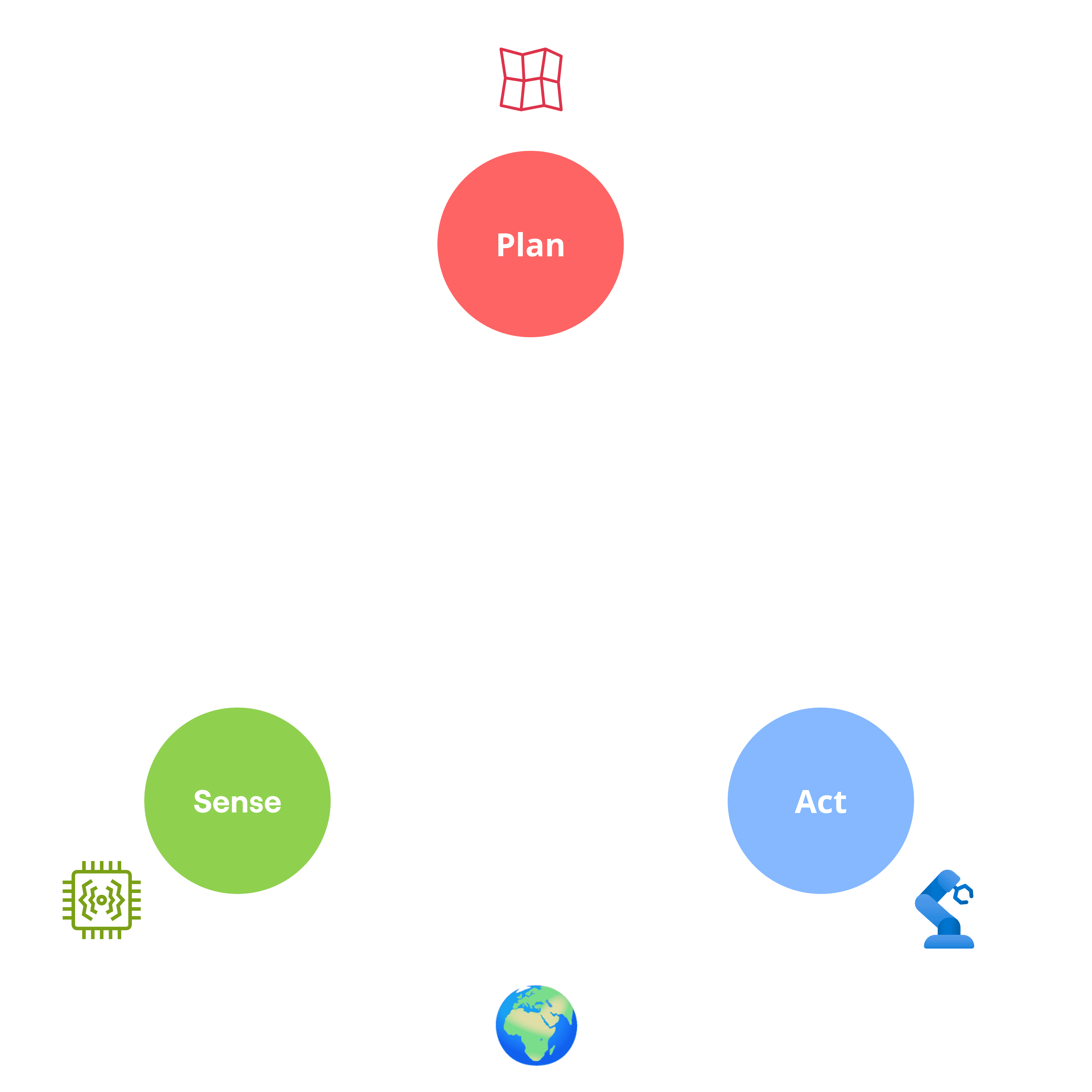
A robot runs the same repeated cycle: sense, plan, act.
Sense is the perception step: the sensors provide readings from the environment, representing the current state of the world, including the robot itself.
Plan is the decision step: these readings are processed and used to plan actions at each timestep until the goal is reached.
Act is the execution step: the decisions are converted into movement by the actuators, the components that drive the joints.
Acting changes the world, and the cycle restarts.
In our example, a position sensor reads the pill and box positions, while the arm reports its own joint angles. The robot plans a trajectory to pick up the pill and place it in the box, then moves the joints to execute the first step of it. If the pill moves, it recomputes the trajectory, and continues until the operation is complete.
A simulated world
The ultimate goal of a simulation is to develop and test that loop without touching hardware. To do this, we swap the world for a simulated one. Sensor readings now come from the simulation itself, and the actuator commands feed back into it, changing its state.
The first piece we need is the simulator. A simulator is the software that holds the representation of the world: all the parameters of the environment, robots and sensors. It continuously runs a loop that updates the world, advancing it in fixed time increments. Each iteration is a timestep. Simulation time does not necessarily match the time it takes to run the simulation: the Real Time Factor (RTF) quantifies this ratio. A simulation can run much faster than real time, reproducing a day's worth of events in a few minutes, or slower if the compute is limited and it struggles to keep up.
The simulator has two main components: the physics engine and the rendering layer.
The physics engine is the core of the simulator. It makes the world evolve according to the laws of physics, modelling gravity, contact forces, collisions and joint dynamics. It is often the most computationally intensive part, so the choice of engine determines how fast the simulation runs and how complex the scenarios can be. Engines range from DART, which runs on CPU and suits smaller scenarios like ours, to PhysX (used in NVIDIA Omniverse), which is GPU-optimised and used for large scenarios such as digital twins of entire warehouses.
The rendering layer produces the visual output. It is how we monitor the simulation at a glance, from multiple points of view, and it is also what camera and other visual sensors read from.
Two commonly used simulators are Gazebo, a lightweight simulator that ships with DART and Ogre2 (rendering) by default, and NVIDIA Isaac Sim, which uses PhysX and the Omniverse RTX renderer. Our example uses Gazebo.
Connecting the components
Even a simple scenario like ours involves sensors, controllers and actuators running as separate pieces. It is good practice to keep them independent and connect them through standard protocols, so that swapping one doesn't affect the rest.
This is what makes the simulation swap possible: the sensors and actuators that interface with the physical world are replaced by simulated versions that read and write the state of the simulation instead, and the planners above them see no difference.
With thousands of robot and sensor types in circulation, real or simulated, there's a need for a common communication interface. This is where ROS (Robot Operating System) comes in: it acts as a message bus between the components. ROS 2 is the current generation, rebuilt on DDS to give distributed real-time publish and subscribe.
The system is split into nodes, independent processes that each handle one piece of the work, and nodes exchange data over topics: named channels that any node can publish to or subscribe to.
In simulation, the connection between the two sides is a component in its own right: the ROS bridge, which publishes the state of the simulated world onto ROS topics and passes commands back the other way.
Sensing
The robot finds out the state of the world, real or simulated, through sensors. In the real world, the robot needs a camera that watches the scene, a detection pipeline that recognises the pill, and a pose estimation framework that uses the camera stream to estimate its position and orientation. The same goes for the box and any other object.
In the simulation, if we're not interested in testing the sensor and the processing of its outputs, we can introduce a fictitious "position sensor" whose output matches our needs: the pill pose. Instead of reproducing the full pipeline, it simply reads the pose from the simulation and republishes it onto a ROS 2 topic. To better imitate a real camera, we restrict the sensor range to a limited area.
Planning
Planning is the step that decides how the arm moves from where it is to where the pill is. The output is a trajectory: a sequence of waypoints, each with a time attached, describing where the arm should be at every moment of the movement. The trajectory has to satisfy several constraints. The joints have speed and acceleration limits, and exceeding them means overshooting the target and stressing the hardware. The path has to avoid the objects in the scene, and the arm has to avoid itself: with six joints there are plenty of configurations where it folds into its own links.
Planning is a well-studied problem. For common cases like ours we don't have to implement it from scratch: frameworks like MoveIt 2 provide a suite of planning algorithms. Given the current and target position, the robot configuration and the constraints, MoveIt 2 plans the trajectory.
In our case, we break the movement into phases: move the arm above the pill, with the gripper pointing down; move the arm down; close the gripper around the pill to grasp it; move the arm above the box; open the gripper. The gripper commands are sent directly without passing through the planner, since they're simple open/close operations.
Joint limits. Tuning the constraints on joint angles is essential. If the limits are too tight, some target positions become unreachable, or reachable only through long, convoluted paths. If the robot is left free to move without limits, planning becomes much harder: it takes longer, and often returns a suboptimal trajectory.
The reason is that there are infinite possible trajectories between two points. The less constrained the robot, the larger that space becomes, and the harder it is for the planner to converge within the planning time budget.
Inverse kinematics. Actuators need the joint angles as input, not coordinates. Inverse kinematics is the step that converts the target pose into the joint angles that reach it.
Control
Once the trajectory is planned, it is passed to a controller that enforces it. The controller is the layer on top of the actuators. It runs continuously, tracking the trajectory against real-time feedback read directly from the joints, because inertia, friction, load and other factors not taken into account at planning time all cause deviations. Separately, a joint_state_broadcaster publishes the state of every joint onto a ROS 2 topic for the rest of the system.
Joints can be controlled in three ways: position, velocity or effort (torque). The choice determines where deviations get corrected. With velocity or effort control, the controller typically corrects them itself, using a PID loop. With position control, the controller sends target positions to the joints, and a lower-level position loop on each joint corrects the error.
In our example, we control the joint angles (position control). A joint_trajectory_controller interpolates between the waypoints and sends target positions to the UR3e, and can stop the movement if the tracking error exceeds set tolerances. A separate JointGroupPositionController commands the gripper. Both come from ros2_controllers, the controller set for ros2_control. In simulation, the lower-level loop is provided by gz_ros2_control, the plugin that connects ros2_control to Gazebo: it sets each joint's velocity in proportion to its position error. On a real arm, this loop typically runs in the robot's own joint controllers.
Controllers can be specific to a robot or a certain part of it, or can be shared across robots. Loading and managing them is handled by a specific component, the controller manager.
Tying it together
Describing the scenario. To describe our scenario to the simulator, there are two types of files: descriptions and configs. Descriptions are .sdf, .srdf and .urdf files, containing definitions of the objects (appearance, physical properties), the world (lighting, physics, object positions etc.), the robot (links, joints, appearance etc.) and the MoveIt semantic layer. Configs specify which controllers exist and their setup, and the planner's parameters.
Starting it up. Everything is collected in a single launch file that starts each piece in parallel. Some components need to be started in order, so the launch file also declares the dependencies.
The full task: two arms, two conveyor belts
Once the pieces are in place, building a more complex scenario is mostly a matter of describing it. We extend the setup to two arms working across two conveyor belts, with objects arriving continuously. This took a new world description, controller configs for the second arm, and a new launch file. The control loop and the sensors stayed as they were.
The one change in the logic is planning, because the targets now move. We estimate each object's velocity and use it to predict its future position. Instead of planning the trajectory for where the object is, we plan it for where it will be, and time it so that the arm reaches the object at the right moment.
What comes next
We started with one arm placing an object in a box and finished with two arms working across two moving conveyor belts. The second scenario built directly on the first, because each component is independent and they communicate through standard protocols.
None of this shows that the system works on a real robot. The physics, timing and sensors are all approximations, and our position sensor skips the camera, detection and pose estimation that a real robot would need. What the simulation has done is narrow down what needs to be proven in the real world.
The next stage is the transfer to real hardware: replacing the simulated sensors and actuators with physical ones, building the perception pipeline, and testing what the simulation can't answer.
Frequently asked questions
What is robotics simulation? Robotics simulation is testing a robot's behaviour in software, using models of the robot, its sensors and its environment. A simulator advances that world in fixed timesteps, with a physics engine working out gravity, contact forces, collisions and joint dynamics. The robot's software reads simulated sensors and sends commands to simulated actuators.
Why simulate a robot instead of testing on real hardware? Real robots are expensive, slow to test and can cause damage or harm. A simulation can run in parallel and faster than real time, compressing months of attempts into a couple of days. Every variable can be controlled, so extreme conditions and corner cases are easy to reproduce with no risk.
How do you simulate a robotic arm? You need a simulator such as Gazebo to model the arm and its environment, ROS 2 to connect the components, a planner such as MoveIt 2 to compute trajectories, and controllers from ros2_control to execute them. Sensors can be simulated in full, or replaced by a position sensor that reads object poses directly from the simulation.
What is the difference between Gazebo and NVIDIA Isaac Sim? Gazebo is a lightweight simulator that uses the DART physics engine and Ogre2 rendering by default. DART runs on CPU and suits smaller scenarios. Isaac Sim uses PhysX and the Omniverse RTX renderer. PhysX is GPU-optimised and used for large scenarios such as digital twins of entire warehouses.
Does behaviour that works in simulation work on a real robot? Not automatically. The physics, the sensors and the timing in a simulation are approximations of reality, so a setup that passes thousands of simulated experiments can still fail the first time it runs on real hardware. Simulation narrows down what needs to be proven in the real world, but it doesn't remove the need to prove it.
Planning a robotics project?
The cheapest time to find out what works is before you commit to hardware. A short roadmap sets out what to test in simulation, what has to be proven on real hardware, and what each step should cost.
We have built a simulation environment for coordinating vehicle fleets and a cooperative drone swarm integrated through ROS. Strategy to production, one team.
